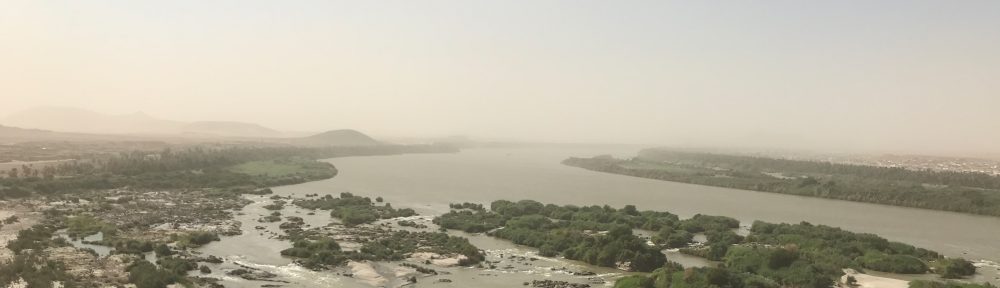
The magnetic data collected at our first campaign in the Attab to Ferka region in 2018/2019 was first processed and interpreted directly after the field season. After the first excavation campaign in 2020, focusing on two of the four geophysically investigated sites, a reconsideration of the data took place. It is based on the excavation results, the photogrammetric data and new kite images.
But before looking at the data, you have to know where exactly on earth the data was generated! The Earth’s magnetic field is a complex system, which is protecting us against ultraviolet radiation, as it is deflecting most of the solar wind, which is stripping away the ozone layer. The earth’s magnetic field can be visualized as a three-dimensional vector: Declination (angle in ° to geographic north, X), Inclination (horizontal angle in ° or magnetic dip, Y) and Intensity (measured in T “Tesla” resp. nT “Nanotesla”, Z). In archaeomagnetism, all components are measured to be compared to the single curves of the region. For magnetometry and interpreting these data, the Inclination is the most important value besides the Declination, which helps for example to detect in situ burnt features. The Inclination describes the angle in which the Earth’s Magnetic Field meets the surface of the Earth itself. Therefore, the angle is changing depending on your position e. g. if you are closer to the magnetic poles or to the magnetic equator.
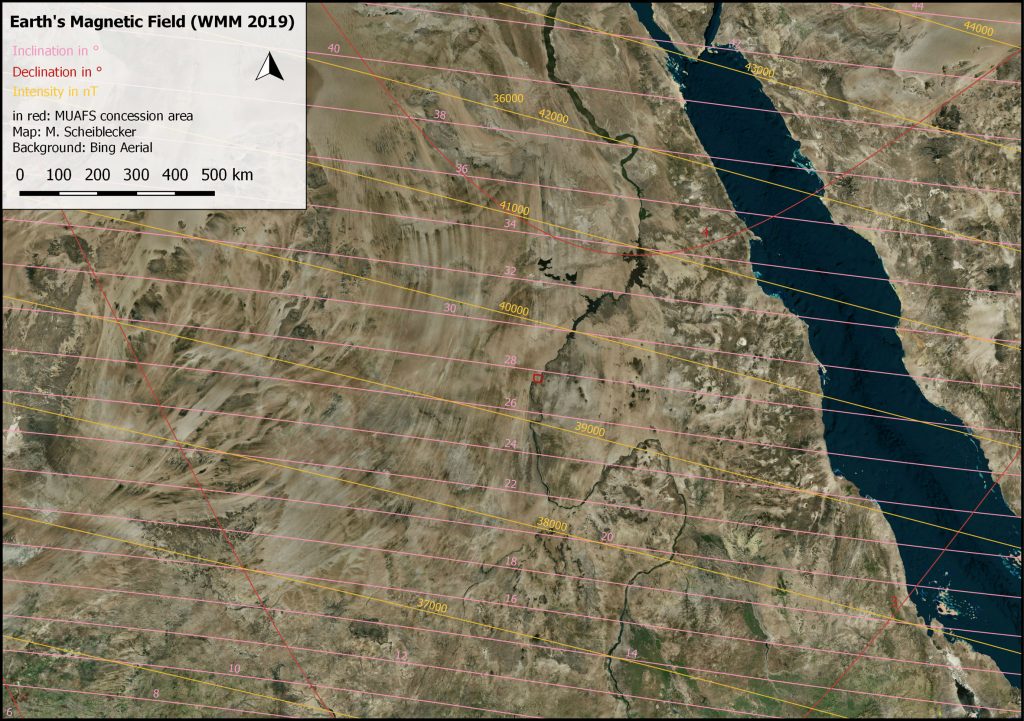
The geomagnetic field changes all the time, every second, every day, and every year! For Munich resp. Fürstenfeldbruck you can follow the alterations simultaneously here. The geomagnetic observatory there is part of the Ludwig-Maximilians-Universität and the Department of Earth and Environmental Studies. As you may know, the magnetic poles are wandering as well. The magnetic north pole did it that fast in the last years that the navigation map had to be changed before the standard interval of five years in 2019. This world magnetic model (WMM) is available online.
But why do we have to know especially the Inclination of the area we are working in and doing magnetometry? The shape and intensity of every single anomaly is depending especially on the Inclination! The shallower the Inclination the wider the anomaly is visible in the magnetogram. Additionally, the dipole (positive/black – negative/white) components are changing. The closer we are measuring to the geomagnetic equator (not the geographic equator), the larger gets the negative part of the anomaly and the lower are the amplitudes of the magnetic signal. Figure 1 illustrates the differences in Inclination for a single anomaly.
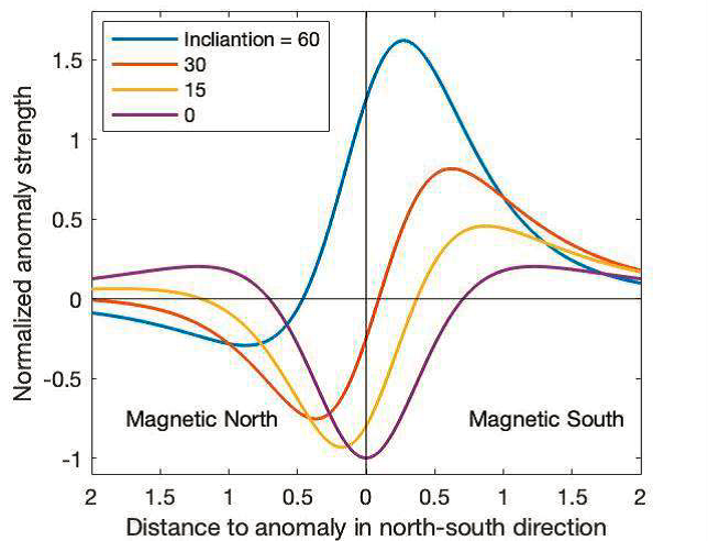
While the Inclination in Munich is around 64°, the Inclination in the MUAFS concession area is 27-28° and shallower. The components of the Earth’s Magnetic Field at the MUAFS concession area are illustrated in Figure 2, showing a Declination of almost 4° and a total field intensity of around 39.000 nT (Munich: 48.585 nT). The measured archaeological and geological features, visible in the magnetogram, are showing contrasts of sometimes less than 1 nT. Due to different Inclinations, the same archaeological feature would result in a different anomaly in Sudan compared to Munich. While the anomaly in Sudan would be wider (see the red curve, Fig. 1) than in Munich (ca. the blue curve, Fig. 1), it would cause lower intensities as well as showing more negative parts than the Munich one. This means while in Bavaria the negative part of an anomaly is regarded more as a small “white shadow”, in Sudan it would be almost equal to the positive part of the anomaly. Furthermore, depending on the depth of the buried feature, the shift in locating the feature could be larger with shallower inclination.
Regarding the used magnetometer – a gradiometer, the intensities are additionally lower than for example with a total field magnetometer, which makes it more difficult to interpret the data and why sometimes low value-features like pisé walls are not detectable with gradiometers. Furthermore, with wider anomalies closer to the geomagnetic equator like in Sudan, it is more possible that anomalies are overlapping so that it is not easy to distinguish features lying next to each other or from different periods.
Usually, magnetograms are shown in greyscale to avoid confusion and “pseudo-limitations” of different values and colors. For interpreting the data, one can play around with the minimum and maximum values as well as inverting of the greyscale version. On magnetograms of measurements with the total field magnetometer usually a high-pass filter is applied, which can be overlayed with the total field data as well.
In rare cases it is helpful to use color scales for the magnetograms additionally to show special features better or to highlight some very high or low values. If the magnetogram is disturbed by high magnetic anomalies like metal fences, iron rubbish on the site etc., color scales are not useful anymore, because they are showing especially the disturbances due to their high amplitudes and less of the archaeological features itself. Nevertheless, it is possible to adjust the color scale as needed for every site separately.
Illustrating the mentioned methods, I would like to show the magnetogram of GiE 002, where a cemetery is located.
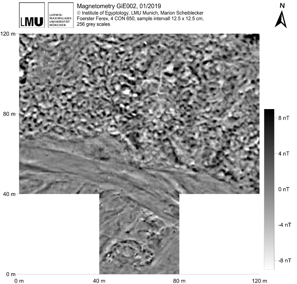
The usual greyscale (Fig. 3) shows clearly the traces of the recent and former wadi/khor, tumuli-like features in the very south as well as lots of features of different shape in the northern part of the magnetogram, interpreted as graves. They are resulting in positive anomalies, accompanied by negative anomalies of different amplitudes.
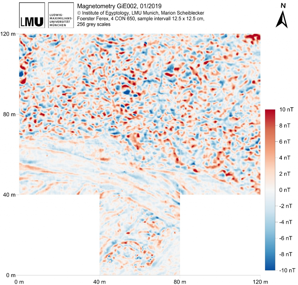
To understand more of the single burials it is helpful to change to a blue-red color scale (Fig. 4). In this way, it is easier to differentiate the single anomalies consisting of the positive (red) and negative (blue) part.
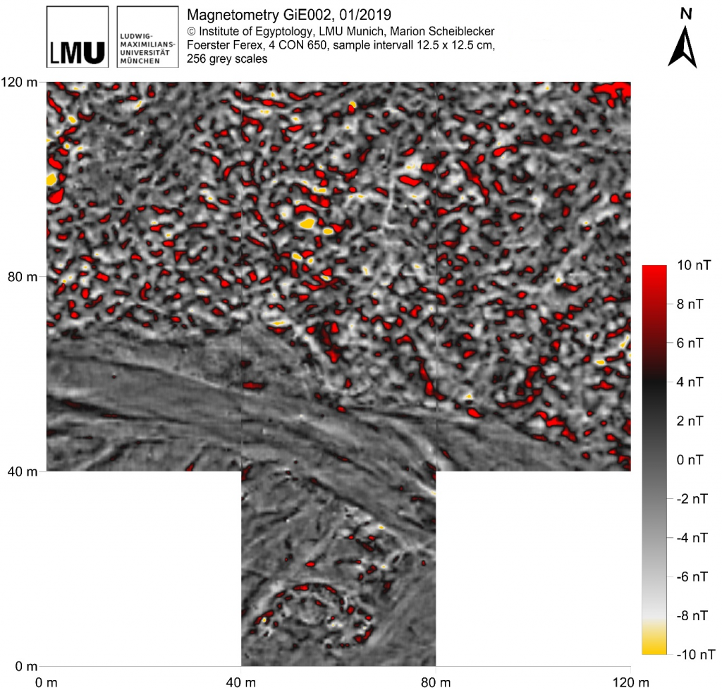
Highlighting the minimum and maximum values – in yellow resp. red – helps e. g. focusing on the probably best-preserved archaeological features located in the center of the measured area, visible in Figure 5.
The magnetograms of GiE 002 show clearly that it is worth playing around with different color scales and that there is more than one magnetogram important for interpreting the data for archaeological and geological purposes.
References
Fassbinder, J. W. E. (2017): Magnetometry for Archaeology. In: Allan S. Gilbert, Paul Goldberg, Vance T. Holliday, Rolfe D. Mandel and Robert Siegmund Sternberg (eds.): Encyclopedia of Geoarchaeology. Dordrecht: Springer Reference (Encyclopedia of Earth Sciences Series), 499-514.
Livermore, P.W.; Finlay, C.C.; Bayliff, M. (2020): Recent north magnetic pole acceleration towards Siberia caused by flux lobe elongation. Nature Geoscience 13, 387–391.
Ostner, S.; Fassbinder, J. W. E.; Parsi, M.; Gerlach, I.; Japp, S. (2019): Magnetic prospection close to the magnetic equator: Case studies in the Tigray plateau of Aksum and Yeha, Ethiopia. In: James Bonsall (ed.): New Global Perspectives on Archaeological Prospection. 13th International Conference on Archaeological Prospection. 28 August – 1 September 2019. Sligo – Ireland. Oxford: Archaeopress, 180-183.