How magnetizable are you? – Magnetization in archaeological prospection

In my latest blog post, I discussed how to read magnetograms and what we have to keep in mind regarding the Earth’s Magnetic Field and the location of the concerning site. Another important factor to approach the comprehensive interpretation of our data is the environment, esp. the geology, geomorphology and formation processes of the region. For magnetometry, it is especially the knowledge about magnetic properties (ferromagnetism) of rocks, minerals and soils.

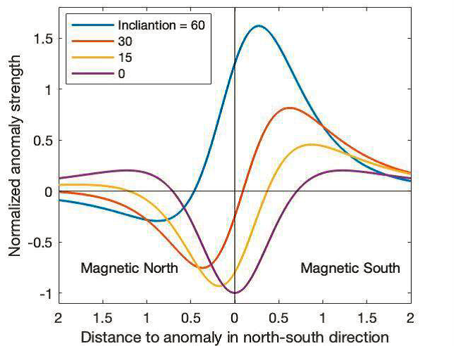
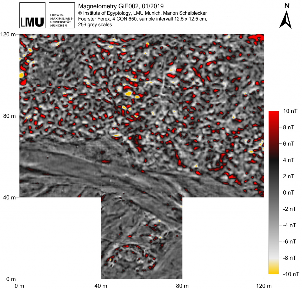
The magnetogram shows the total magnetization, which is composed by the induced and the remanent magnetization (Fig. 1). The relation of induced and remanent magnetization is described by the Koenigsberger ratio (Q-ratio). It informs us not only about the quality of the rock sample for paleomagnetism, but also if we are dealing with archaeological objects.

Figure 1: Magnetization for rocks with induced and remanent amounts (Lowrie 2007, 321 fig. 5.40 a).

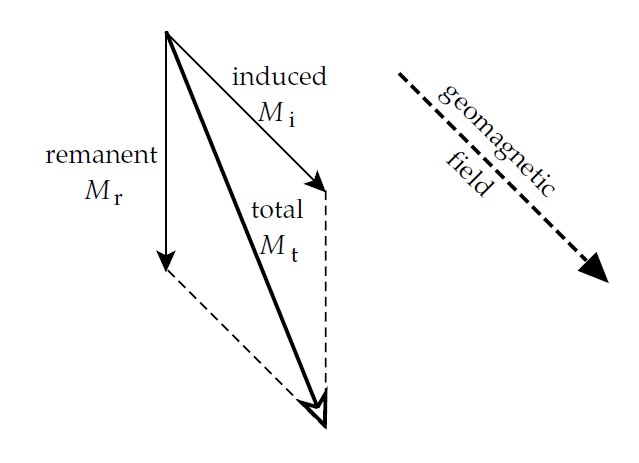
The induced magnetization exists with an applied external field only, e.g. the Earth’s Magnetic Field, and mostly goes along with the direction of the Earth’s Magnetic Field. For interpreting our magnetograms, it is helpful to conduct additional magnetic susceptibility measurements in the field, which tells us more about the induced magnetization. The magnetic susceptibility describes how magnetizable a sample/material is in an applied field. It is affected by the type of contained minerals as well as their grain size. The resulting values are unit less and can be negative (diamagnetic) or positive (ferromagnetic, ferrimagnetic, paramagnetic). Susceptibility can be measured in the field as well as in the laboratory, where more precise measurements are possible and additional parameter can be investigated.

The remanent magnetization is a permanent magnetization, independent of an external field, and important in paleomagnetism and archaeomagnetism. The natural remanent magnetization is the sum of the remanent magnetization and can be composed by several elements. For archaeological prospection, one of the most important remanent magnetizations is the thermoremanent magnetization (TRM). It is formed through heating of material over Curie temperature and cooling in an applied magnetic field, whose direction (Declination) is saved. Kilns, ovens and burnt objects like pottery or bricks etc. are the best examples for TRM. Chemical remanent magnetization (CRM) can be found in sedimentary or metamorphic rocks, whereas detrital remanent magnetization (DRM) develops during sedimentation of small magnetic particles in smooth water. Isothermal remanence (IRM) is the reason why we can detect also lightning strikes (LIRM) in our magnetograms. Although remanent magnetization is usually permanent, several factors could alter it, such as weathering.

But why are some materials/rocks more magnetic or magnetizable than others? It depends on iron oxides. Iron oxides are not only responsible for magnetization but also playing a role which colour a material has. The most important iron oxides regarding archaeological purposes are magnetite, maghemite, greigite, hematite, goethite as well as titanomagnetites, occurring in soils. While magnetite and maghemite are showing up to 1000 times higher susceptibilities than hematite, the latter is responsible for the typical red colour. Pedogenic, anthropogenic, lithogenic, and bacterial processes are responsible for the enhancement of soils, esp. top soils. Additionally, originally nonmagnetic materials can show enhanced magnetization: magnetotactic bacteria in organic materials are generating magnetite so that already gone posts, palisades etc. can be detected by magnetometry.

Magnetic susceptibility measurements in the field can be carried out selective e.g. for scattered objects and rocks on the surface or areal (separate geophysical prospection method). They can be used to define the extension of archaeological sites, activity zones or features in human made environments. Furthermore, they help understanding the morphology, formation processes, erosion and sedimentation as well as stratigraphic sequences for climate research and soil formation processes. Usually, top soils as well as archaeological soils are showing higher magnetic susceptibility values caused by enhancement of magnetic minerals due to the use of fire and fermentation. That is the reason why we can detect areas of human activity, e.g. settlements, and determine their extension.

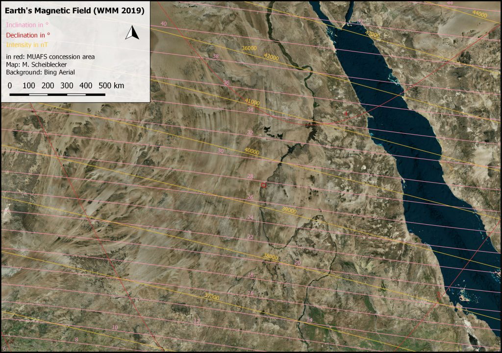
How can we transfer this knowledge to the MUAFS concession area? The geological map of the Nile valley shows mostly sandstones, siltstones and mudstones accompanied by metavolcanic rocks as well as colluvium, sand sheets and dunes. For the volcanic rocks, we can assume high magnetic susceptibilities, whereas for the sandstones, siltstones and mudstones weak magnetic susceptibility is rather likely, depending on the contained minerals.

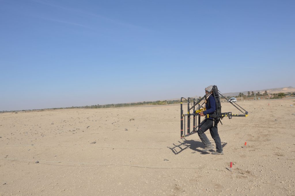
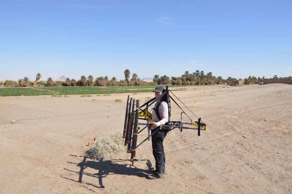
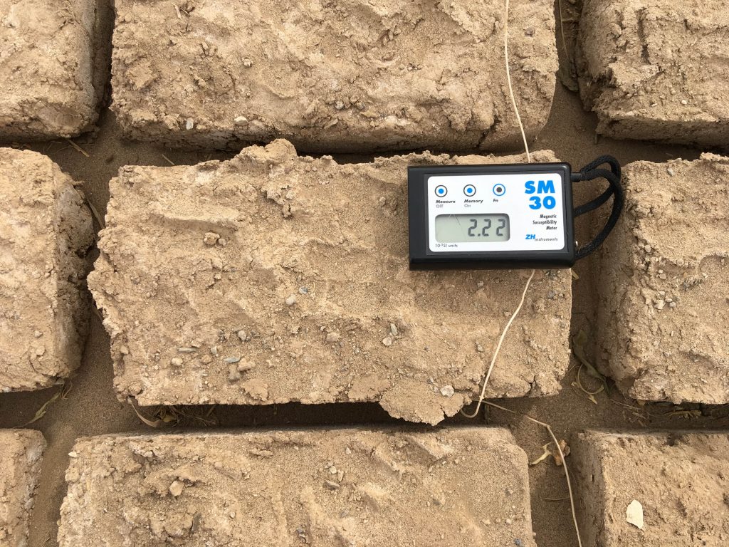
During the first geophysical campaign, we conducted spotty magnetic susceptibility measurements on our sites as well as the environment. Therefore, we used the handheld Kappameter SM-30 (Zh-instruments, Fig. 2). While magnetometry is a passive method, magnetic susceptibility meter are active instruments with a small coil included. Sampling the scattered rocks and archaeological objects like mudbricks gives an idea what we can expect in the magnetogram. Furthermore, the method can be applied in excavation trenches e.g. to distinguish stratigraphic layers or walls/floors and susceptibility maps can be produced. Due to magnetic susceptibility it is feasible to differentiate sources of raw material e.g. for mudbricks.

Figure 2: Measuring the magnetic volume susceptibility of a mudbrick laid out in the sun for drying with the Kappameter SM-30, showing a value of 2.22 [10-3 SI] (M. Scheiblecker).

For the settlement site GiE 001 at Ginis East, the scattered rock material shows mostly susceptibility values in a range of 0,302 to 0,826 [10-3 SI], esp. quartz, schist, and sedimentary rocks, while rocks of volcanic origin result in values around 7,5 [10-3 SI]. The surface values are ranging between 4,35 to 5,6 [10-3 SI] and mudbrick from a partly upright standing hut shows values of around 4 [10-3 SI]. For this site, we could expect therefore the following: walls made of sedimentary rocks would cause negative anomalies in the magnetogram, while the use of volcanic rock would result in positive anomalies. Mudbrick or galus walls (of stamped mud) are more difficult to predict; depending on their mineral composition, they are revealing positive or negative anomalies. Fire installations or the use of fired bricks would be easily recognizable because of their high values.

A profile along a street close to the Nile River shows the different sedimentation layers very nicely: different colours as well as susceptibility values can be seen in Figure 3.

Figure 3: Magnetic susceptibility values (in 10-3 SI) of a profile next to the Nile (M. Scheiblecker).

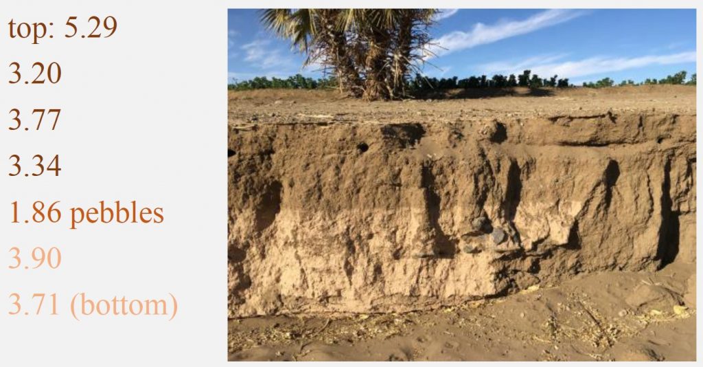
This example shows the complexity of magnetic susceptibility in combination with colours; darker and brighter layers show similar values, whereas the surface reaches the highest value. The layer with pebbles reveals the lowest value due to the included pebbles of probably sedimentary origin. For understanding the environment of archaeological sites and their formation processes, it is important to consider not only the survey, excavation and magnetometry results itself. Furthermore, knowledge in geology, geomorphology as well as the investigation of their parameters add details for a comprehensive picture of an archaeological landscape.

At the end, if you are asking yourself how magnetizable you are: without any ferromagnetic items from your clothes or e.g. glasses, the magnetic susceptibility would be almost zero or even negative, as the human body consists mostly of water.

References

Aspinall, A.; Gaffney, C.F.; Schmidt, A. (2008): Magnetometry for Archaeologists. Geophysical methods for archaeology 2. Lanham: AltaMira Press.

Butler, R.F. (1998): Paleomagnetism: Magnetic Domains to Geologic Terranes: Electronic Edition. Boston: Blackwell.

Dalan, R. (2017): Susceptiblity. In: Allan S. Gilbert, Paul Goldberg, Vance T. Holliday, Rolfe D. Mandel and Robert Siegmund Sternberg (eds.): Encyclopedia of Geoarchaeology. Dordrecht: Springer Reference (Encyclopedia of Earth Sciences Series), 939–944.

Fassbinder, J.W.E.; Stanjek, H.; Vali, H. (1990): Occurrence of Magnetic Bacteria in Soil. Nature 343 (6254), 161–163.

Fassbinder, Jörg W. E. (2017): Magnetometry for Archaeology. In: Allan S. Gilbert, Paul Goldberg, Vance T. Holliday, Rolfe D. Mandel and Robert Siegmund Sternberg (eds.): Encyclopedia of Geoarchaeology. Dordrecht: Springer Reference (Encyclopedia of Earth Sciences Series), 499–514.

Lowrie, W. (2007): Fundamentals of Geophysics, Cambridge: Cambridge University Press.

More than greyscale: How to read magnetograms in the MUAFS concession area

The magnetic data collected at our first campaign in the Attab to Ferka region in 2018/2019 was first processed and interpreted directly after the field season. After the first excavation campaign in 2020, focusing on two of the four geophysically investigated sites, a reconsideration of the data took place. It is based on the excavation results, the photogrammetric data and new kite images.

But before looking at the data, you have to know where exactly on earth the data was generated! The Earth’s magnetic field is a complex system, which is protecting us against ultraviolet radiation, as it is deflecting most of the solar wind, which is stripping away the ozone layer. The earth’s magnetic field can be visualized as a three-dimensional vector: Declination (angle in ° to geographic north, X), Inclination (horizontal angle in ° or magnetic dip, Y) and Intensity (measured in T “Tesla” resp. nT “Nanotesla”, Z). In archaeomagnetism, all components are measured to be compared to the single curves of the region. For magnetometry and interpreting these data, the Inclination is the most important value besides the Declination, which helps for example to detect in situ burnt features. The Inclination describes the angle in which the Earth’s Magnetic Field meets the surface of the Earth itself. Therefore, the angle is changing depending on your position e. g. if you are closer to the magnetic poles or to the magnetic equator.

The geomagnetic field changes all the time, every second, every day, and every year! For Munich resp. Fürstenfeldbruck you can follow the alterations simultaneously here. The geomagnetic observatory there is part of the Ludwig-Maximilians-Universität and the Department of Earth and Environmental Studies. As you may know, the magnetic poles are wandering as well. The magnetic north pole did it that fast in the last years that the navigation map had to be changed before the standard interval of five years in 2019. This world magnetic model (WMM) is available online.

But why do we have to know especially the Inclination of the area we are working in and doing magnetometry? The shape and intensity of every single anomaly is depending especially on the Inclination! The shallower the Inclination the wider the anomaly is visible in the magnetogram. Additionally, the dipole (positive/black – negative/white) components are changing. The closer we are measuring to the geomagnetic equator (not the geographic equator), the larger gets the negative part of the anomaly and the lower are the amplitudes of the magnetic signal. Figure 1 illustrates the differences in Inclination for a single anomaly.

Figure 1: Anomaly strength of the total field intensity as north-south traverse through the anomaly’s centre for different Inclinations (Ostner et al. 2019, 181 Fig. 2).

While the Inclination in Munich is around 64°, the Inclination in the MUAFS concession area is 27-28° and shallower. The components of the Earth’s Magnetic Field at the MUAFS concession area are illustrated in Figure 2, showing a Declination of almost 4° and a total field intensity of around 39.000 nT (Munich: 48.585 nT). The measured archaeological and geological features, visible in the magnetogram, are showing contrasts of sometimes less than 1 nT. Due to different Inclinations, the same archaeological feature would result in a different anomaly in Sudan compared to Munich. While the anomaly in Sudan would be wider (see the red curve, Fig. 1) than in Munich (ca. the blue curve, Fig. 1), it would cause lower intensities as well as showing more negative parts than the Munich one. This means while in Bavaria the negative part of an anomaly is regarded more as a small “white shadow”, in Sudan it would be almost equal to the positive part of the anomaly. Furthermore, depending on the depth of the buried feature, the shift in locating the feature could be larger with shallower inclination.

Figure 2: The Earth’s Magnetic Field in Sudan after World Magnetic Model (WMM) 2019, with the MUAFS concession area in red (M. Scheiblecker).

Regarding the used magnetometer – a gradiometer, the intensities are additionally lower than for example with a total field magnetometer, which makes it more difficult to interpret the data and why sometimes low value-features like pisé walls are not detectable with gradiometers. Furthermore, with wider anomalies closer to the geomagnetic equator like in Sudan, it is more possible that anomalies are overlapping so that it is not easy to distinguish features lying next to each other or from different periods.

Usually, magnetograms are shown in greyscale to avoid confusion and “pseudo-limitations” of different values and colors. For interpreting the data, one can play around with the minimum and maximum values as well as inverting of the greyscale version. On magnetograms of measurements with the total field magnetometer usually a high-pass filter is applied, which can be overlayed with the total field data as well.

In rare cases it is helpful to use color scales for the magnetograms additionally to show special features better or to highlight some very high or low values. If the magnetogram is disturbed by high magnetic anomalies like metal fences, iron rubbish on the site etc., color scales are not useful anymore, because they are showing especially the disturbances due to their high amplitudes and less of the archaeological features itself. Nevertheless, it is possible to adjust the color scale as needed for every site separately.

Illustrating the mentioned methods, I would like to show the magnetogram of GiE 002, where a cemetery is located.

Figure 3: Magnetogram of GiE 002 in greyscale (M. Scheiblecker).

The usual greyscale (Fig. 3) shows clearly the traces of the recent and former wadi/khor, tumuli-like features in the very south as well as lots of features of different shape in the northern part of the magnetogram, interpreted as graves. They are resulting in positive anomalies, accompanied by negative anomalies of different amplitudes.

Figure 4: Magnetogram of GiE 002 in blue to red color scale (M. Scheiblecker).

To understand more of the single burials it is helpful to change to a blue-red color scale (Fig. 4). In this way, it is easier to differentiate the single anomalies consisting of the positive (red) and negative (blue) part.

Figure 5: Magnetogram of GiE 002 in highlighted grey scale, showing maximum values in red as well as minimum values in yellow (M. Scheiblecker).

Highlighting the minimum and maximum values – in yellow resp. red – helps e. g. focusing on the probably best-preserved archaeological features located in the center of the measured area, visible in Figure 5.

The magnetograms of GiE 002 show clearly that it is worth playing around with different color scales and that there is more than one magnetogram important for interpreting the data for archaeological and geological purposes.

References

Fassbinder, J. W. E. (2017): Magnetometry for Archaeology. In: Allan S. Gilbert, Paul Goldberg, Vance T. Holliday, Rolfe D. Mandel and Robert Siegmund Sternberg (eds.): Encyclopedia of Geoarchaeology. Dordrecht: Springer Reference (Encyclopedia of Earth Sciences Series), 499-514.

Livermore, P.W.; Finlay, C.C.; Bayliff, M. (2020): Recent north magnetic pole acceleration towards Siberia caused by flux lobe elongation. Nature Geoscience 13, 387–391.

Ostner, S.; Fassbinder, J. W. E.; Parsi, M.; Gerlach, I.; Japp, S. (2019): Magnetic prospection close to the magnetic equator: Case studies in the Tigray plateau of Aksum and Yeha, Ethiopia. In: James Bonsall (ed.): New Global Perspectives on Archaeological Prospection. 13th International Conference on Archaeological Prospection. 28 August – 1 September 2019. Sligo – Ireland. Oxford: Archaeopress, 180-183.

Finding solutions: The first magnetometry campaign in the Attab to Ferka region

Following up my last blog entry I would like to provide you an insight into the first archaeological prospection campaign almost two years ago, the work in the field and our challenges.

The first geophysical campaign in the Attab to Ferka region included magnetometry as well as magnetic susceptibility measurements. It took place during the first MUAFS season in December 2018/January 2019 and covered more than 6 ha at four different sites on the East bank of the Nile (GiE001 – GiE004).  Our grid system for magnetic measurements consists of 40 x 40 m squares, which were staked out using a right-angle prism, measuring tapes and ranging poles. The advantage of staking out by hand is that we could perfectly orientate our grid system regarding the site and its visible traces as well as the topography. Excepting some quartz outcrops, burial mounds, dense bushes and deep wadis, staking out and walking with the magnetometer was feasible.

For every grid corner we were using wooden sticks to fix our marked base lines for the measurements. For taking magnetic measurements we used the Foerster Ferex 4.032 Gradiometer (65 cm Gradient) in handheld Quadro-sensor configuration. The grids are measured in zig-zag mode every 2 m to reach a spatial coverage of 0,5 x 0,125 m. It is important not to use ferromagnetic pieces for the instrument, that’s why the frame is completely non-magnetic. Furthermore, the measuring person as well as the helping people around are not wearing magnetic clothes/accessories.

Magnetic measurements using 40 x 40 m grids and 2 m separated marked ropes for the zig-zag mode at GiE 002 in 2019 (Photo: Giulia D’Ercole).

Not only the measuring equipment and person have to be non-magnetic, there shouldn’t be magnetic disturbances in the surrounding area as well, for example streets, train, powerlines etc. Their noise is affecting the measurements and at its worst making them impossible or useless. Our investigated sites were suitable for magnetic measurements; solely the pillars of the powerline were disturbing the measurements in the direct surrounding of the pillars at our first site.

But there were other challenges: strong winds during our campaign made it quite difficult to stake out the grids properly. That’s why it took longer as usual and influenced also the communication as you couldn’t understand each other standing 40 m apart. Additionally, it was quite tricky to walk straight, with the same speed and with a constant distance between the probes and the ground (ideally 30 cm). It was not only more time consuming but also taking more strength to do the measurements in that windy, squally surrounding and also to avoid vibrations of the bag-pack and the magnetometer frame, which would affect the measurements.

A crucial part of fieldwork though is the exact positioning of the investigated areas! As magnetometry is a passive method, you can repeat the measurements as often as needed. Using precise positioning you can come back to specific spots you are interested in. For example, excavation trenches can be specified easily avoiding time consuming and expensive large area trenches. Furthermore, archaeological survey results can be combined, at best including dating of architectural features. Altogether it is feasible to follow special issues and questions regarding the micro and macro region of sites.

To georeference our magnetic data we took the coordinates of every wooden stick marking the corners of the grids. Therefore, we were using our dGPS (Differential Global Positioning System). As no official benchmarks are available in the Attab to Ferka region new fixpoints were set. The advantage is that we can use them not only for surveys but also for integrating the excavation trenches into our GIS-projects.

Unfortunately, several of our benchmarks set in 2018/2019 and embedded in concrete were missing when coming back to the region for the excavation campaign in early 2020. That’s why a quick solution had to be found to use the created measurement grid further on, where not only the benchmarks and survey points were integrated, but also the data collected during drone mapping and magnetic survey. A fictive grid was set up based on the remaining benchmarks to embed the new excavation trenches and their photogrammetry data.

Our challenge now is to merge both datasets to be able to compare the excavated features with all collected magnetic data as well as our high-resolution drone images. This allows to verify the magnetometry results and learn more for new measurements in future.

On the tracks of ancient cultures: Archaeological Geophysics

As a team member of the first MUAFS season 2018/2019 responsible for magnetic investigations I would like to introduce the geophysical methods used for archaeological purposes. These methods will also be highly relevant for the DiverseNile project.

In the last decades, geophysics became a substantial part of archaeological projects. Depending on several factors, the most suitable geophysical method is chosen: the environment (desert, steppe, swampland etc.), the archaeological period and the used archaeological materials (stone, mudbrick etc.), but also the questioning (settlement layout and extension, cemetery detection etc.).  Additionally, the decision is influenced by available time, financial means and sometimes the season.

Still the fastest and most effective geophysical method in archaeology is magnetometry. It provides getting an overview of a site as well as its environment, extension and layout. Magnetic prospecting enables us to distinguish between settlement and burial sites, their structure, special buildings, open areas, as well as fortifications. Depending on the chosen sensors, we can learn more about the geology and environment and their changes over time. Accompanying measurements of magnetic susceptibility deliver information about magnetic properties of scattered objects and building materials as well as archaeological sediments and can be used in archaeological excavations as well.

Magnetic gradient investigations in Ginis 2019, site GiE 001 (Photo: Giulia D’Ercole).

But how does it work? Magnetometers are recording the intensity of the earth magnetic field with high-resolution. Nowadays, the earth magnetic field in the Attab to Ferka region has an intensity of around 39.400 Nanotesla (nT). With sensitive total field magnetometers, magnetic anomalies of less than 1 nT can be detected during archaeo-geophysical surveys, displaying even archaeological features like mudbrick walls or palisades.

Magnetic investigations benefit from varying magnetic properties of archaeological soils and sediments as well as materials. Every human activity regarding the surface is detectable because of different magnetic response. For example, digging a ditch, building a wall or using a kiln is changing or disturbing the actual earth magnetic field. What else can be detected? Architecture, streets, canals and riverbeds, ditches, pits and graves can be revealed just as palisades, posts and fire installations. Additionally, more information about geological and environmental conditions can be collected using magnetometry, e. g. paleo channels or former wadis.

For detecting stone architecture and for example voids, resistivity (areal or profile) and Ground Penetrating Radar (GPR) methods are applied, partly in addition to magnetic investigations. While magnetometry gives an overview about buried features beneath the surface in a ‘timeless picture’, GPR and ERT (Electrical Resistivity Tomography) provide more information about the depth and preserved height of the features. Of course, more than one geophysical method can be applied to get a comprehensive dataset for more complete interpretation of the results. Combined with archaeological work – survey and excavation – we can increase our knowledge and understanding of physical properties of archaeological and geological features as well as improve our interpretation.

Geophysical prospecting was originally developed for military purposes to detect submarine boats, aircrafts or gun emplacements. Furthermore, natural and especially mineral resources can be located. Geophysical methods and first of all magnetometry are used in archaeology since the late 1950s, when Martin Aitken detected Roman kilns in the UK. In Sudan, magnetometry is used since the late 1960s when Albert Hesse started investigations at Mirgissa in Lower Nubia. Since then, instruments as well as software programs for data collecting, processing and imaging have been developed and improved and offer detailed mapping of sites. First, geophysical prospecting can be applied fast, nondestructive and comprehensive. For magnetic prospection there is a variety of configurations to use, from handheld one/two-sensor instruments to motorized and multisensory systems but also different types of sensors. Through geographic information systems (GIS) geophysical investigations are benefiting from integrating high-resolution satellite images, drone images and models, survey and excavation data for a comprehensive interpretation of results.

After collecting magnetic data in the field, the files are downloaded and processed to get an idea of the first results. With that the field measurement proceeding can be adjusted as well as excavation trenches can be chosen. The detailed processing and analyzing of the collected field data are conducted back home on the desk.

References

Campana, Stefano; Piro, Salvatore (eds.) (2009): Seeing the Unseen. Geophysics and Landscape Archaeology. London: Taylor & Francis.

Dalan, R. (2017): Susceptiblity. In: Allan S. Gilbert, Paul Goldberg, Vance T. Holliday, Rolfe D. Mandel and Robert Siegmund Sternberg (eds.): Encyclopedia of Geoarchaeology. Dordrecht: Springer Reference (Encyclopedia of Earth Sciences Series), 939–944.

Fassbinder, Jörg W. E. (2017): Magnetometry for Archaeology. In: Allan S. Gilbert, Paul Goldberg, Vance T. Holliday, Rolfe D. Mandel and Robert Siegmund Sternberg (eds.): Encyclopedia of Geoarchaeology. Dordrecht: Springer Reference (Encyclopedia of Earth Sciences Series), 499–514.

Herbich, Tomasz (2019): Efficiency of the magnetic method in surveying desert sites in Egypt and Sudan: Case studies. In: Raffaele Persico, Salvatore Piro and Neil Linford (eds.): Innovation in Near-Surface Geophysics. Instrumentation, Application, and Data Processing Methods. First edition. Amsterdam, Oxford, Cambridge: Elsevier, 195–251.

Schmidt, Armin; Linford, Paul; Linford, Neil; David, Andrew; Gaffney, Chris; Sarris, Apostolos; Fassbinder, Jörg (2015): EAC Guidelines for the Use of Geophysics in Archaeology. Questions to Ask and Points to Consider. Namur: Europae Archaeologia Consilium (EAC Guidelines, 2).